You can see your final score (out of 15) for the assignment on Moodle. In addition, you can view the feedback on the assignment, which explains some of the issues, the marking scheme and gives detailed notes on the marks received by each group. Also you can view reports of two of the groups that received top marks (group 14 and group 22). By comparing your report with theirs you will get a better idea of why you may not have received full marks.
Note that if you tried 4 values for each parameter (e.g. 4 different uplink data rates, 4 different RTTs) then the maximum experiments for "No errors" is 4 x 4 x 4 x 4 = 256. And "with errors" since the window size is always 1 the maximum number of experiments is 4 x 4 x 4 x 1 x 4 x 4 = 1024. I don't expect you to run 1280 experiments, nor must you use only 4 values for each parameter. So you should select the parameters values to use that will show the important trends but also keep the number of experiments to something you can perform in reasonable time.
Form a group of 3 students. You may mix between IT and CS. Masters and Exchange students may either form a group of 2 or a group of 3. Masters students should NOT mix with non-Masters students.
Groups are:
A summary of the steps for the assignment follow. Details of steps are either described in the links or below.
virtnet uses VirtualBox to create Linux virtual machines that are automatically configured in a desired network topology. It is just a set of scripts I created to allow easy/quick setup of the virtual machines, configuration of the network interfaces, and also includes tools/software often useful for learning about Linux, networking and security.
You can run virtnet on your own computer (it has been tested on Windows 7, OSX, and Ubuntu Linux) or on a lab computer (some of the Macs on the 3rd floor already have it installed).
Instructions for installing/using are available at: http://sandilands.info/sgordon/automatic-creation-of-virtual-network-with-vboxmanage
Some basic troubleshooting is available. If you have problems using virtnet, then take a screenshot of the error and send it in an email to me, including a brief description of the problem and OS you are using (e.g. OSX, Windows 8).
I have created some very simple Python applications that implement:
Your main goal is to experiment with these, analyzing the performance of each under different link conditions. The implementation is specific for this assignment, and in particular for the use on virtnet. There is some code included to make it slightly easier to analyse when using virtnet, but means the code is not very good for real networks.
The following is an example of performing an experiment, in this case with stop-and-wait flow control, with data going from node1 to node2.
As the performance of flow/error control depends on the link characteristics, we must first set them. Lets set the link from node1 to node2 to have a data rate of 1 Mb/s and a delay of 10 ms. And the return link we will set the data rate to 100 Mb/s with 0 ms delay.
+-------+                          +-------+
|       | ===== 1Mb/s, 10ms =====> |       |
| node1 |                          | node2 |
|       | <==== 100Mb/s, 0ms ===== |       |
+-------+                          +-------+
To set the link characterstics you should use vn-link, as described here.
For this assignment you should always set the return link (node2 to node1) to be 100 Mb/s and 0 ms. The high data rate means ACKs will have a very small transmission delay - we can almost ignore them. The 0 ms delay just means you only have to modify the link delay from node1 to node2 to set the round-trip-time (RTT).
Once you have set the link characteristics, start the arq_server on node2, and then start arq_client on node1. Below is an example of the commands on both nodes, including setting the link data rate and delay with vn-link and then running the client and server. First on node2, the server:
network@node2:~$ sudo bash ~/virtnet/bin/vn-link --interface eth1 --set --rate 100000kbit --delay 0ms
Old values
  Rate: not set
  Delay: not set
  Jitter: not set
RTNETLINK answers: No such file or directory
New values
  Rate: 100000kbit
  Delay: 0ms
  Jitter: not set
network@node2:~$ cd virtnet/src/sockets/
network@node2:~/virtnet/src/sockets$ python arq_server.py 100 10000 1 1 0.0
Duration: 11.752507925
OriginalPacketsReceived: 100
AcksSent: 100
TotalDataReceived:  1000000
TotalBytesReceived: 1000000
TotalBytesReceivedIncHeaders: 1470000
Errors: 0
ReceiveRate: 125079.685917
Throughput: 85088.2217122
100 , 10000 , 1 , 11.752507925 , 100 , 100 , 1000000 , 1000000 , 1470000 , 0 , 125079.685917 , 85088.2217122 ,
And node1, the client:
network@node1:~$ sudo bash ~/virtnet/bin/vn-link --interface eth1 --set --rate 1000kbit --delay 10.0ms
Old values
  Rate: not set
  Delay: not set
  Jitter: not set
RTNETLINK answers: No such file or directory
New values
  Rate: 1000kbit
  Delay: 10.0ms
  Jitter: not set
network@node1:~$ cd virtnet/src/sockets/
network@node1:~/virtnet/src/sockets$ python arq_client.py 100 10000 1 4 1.0
0.000012875 LastSeqTx 0 LastAckRx 65535 CurWin 1
0.000201941 StartTime 1414297056.0 DataLength 10000
0.000272036 TxData 0 DataLength 10000
0.000959873 LastSeqTx 0 CurWin 0
0.116370916 RxAck 1
0.116510868 LastAckRx 1 CurWin 1
0.116571903 TxData 1 DataLength 10000
0.117251873 LastSeqTx 1 CurWin 0
0.232434034 RxAck 2
0.232585907 LastAckRx 2 CurWin 1
...
11.528374910 TxData 98 DataLength 10000
11.529227972 LastSeqTx 98 CurWin 0
11.647837877 RxAck 99
11.647974014 LastAckRx 99 CurWin 1
11.648031950 TxData 99 DataLength 10000
11.648675919 LastSeqTx 99 CurWin 0
11.765501022 RxAck 100
11.765655041 LastAckRx 100 CurWin 1
Duration: 11.765709877
OriginalPacketsSent: 100
RetransmittedPacketsSent: 0
AcksRecevied: 100
BytesAcked: 1000000
TotalDataSent: 1000000
TotalBytesSent: 1050000
TotalBytesSentIncHeaders: 1470000
SendingRate: 124939.337734
Throughput: 84992.7467576
100 , 10000 , 1 , 1.0 , 11.765709877 , 100 , 0 , 100 , 1000000 , 1000000 , 1050000 , 1470000 , 124939.337734 , 84992.7467576 ,
The options select for the client and server:
The output from the programs finishes with useful statistics, first named line-by-line, and then the last line includes the same values but in a comma-separated format (so you can easily copy-and-paste into a spreadsheet).
Now you can try the same protocol but with different link conditions, and/or change the protocol parameters (e.g. different data size, window).
Once you have installed virtnet and can run the arq_client and arq_server Python applications (and understand the parameters and output), you should plan and run a set of experiments. The aim of the experiments are to understand:
You can do this by repeatedly running the client and server with different link characteristics and protocol parameters. The parameters that you may vary, and some suggested values include:
You should "intelligently" select parameter values. That is, don't just try every possible value. Instead think about the values which will produce results that indicate trends.
Each time you run the client/server you will get some results. The main result of interest is the measured throughput. You should record the measured throughput at the server (due to the implementation, it is more accurate at the server than that reported at the client) and then convert into efficiency. As you change parameters, you should observe how those changes impact on the measured efficiency. Then you should plot the results from multiple experiments. In addition, you should plot the expected efficiency. You must calculate the expected efficiency from the link conditions and protocol parameters (and your knowledge of stop-and-wait and sliding window).
An example plot might look like this (of course, yours will be created with a computer, not drawn by hand, will include data points, may use different line/plot styles - i.e. yours will look much better than this):
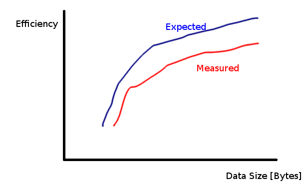
That is, you will show how the performance (efficiency) changes as the parameter (data size) changes, both from your experimental (measured) values and your calculated (expected) values.
Then you will produce plots of efficiency vs other parameters.
An important aspect is that the measured values are statistically significant. In this assignment, that means that you run the experiments for enough packets. Recall that the first parameter of arq_client and arq_server is the number of original data frames to send. This should be at least 100, and in cases when there are errors, closer to 1000. Otherwise the average values reported may not be an accurate representation of the true values.
Several students have asked "how many experiments must they perform?". There is no one correct answer: it may range from 10's of experiments to 100's of experiments. The best way to know if you have enough is to plot the results as you collect them. What you should see is:
The 2nd point is evident when changing the window size. Some students have performed experiments with different window sizes but obtain about the same efficiency. I will explain what causes this in the following.
The efficiency of sliding window mainly depends on: DATA transmission time, propagation time (to B and back) and window size. If you choose "appropriate" values of DATA transmission time (depends on data size and data rate) and propagation time (the delay from A to B, since in the experiments you set the delay from B to A to 0), then you should see changes of efficiency as the window size changes (at least for several values of window size). What are "appropriate" values of transmission and propagation time? Consider the following example where the transmission time is much larger than the propagation time. Here is the timing diagram for window of 1 and 2 (note in your experiments you should NOT use a window of 2; it should be 1, 3, 7, 15, ...).
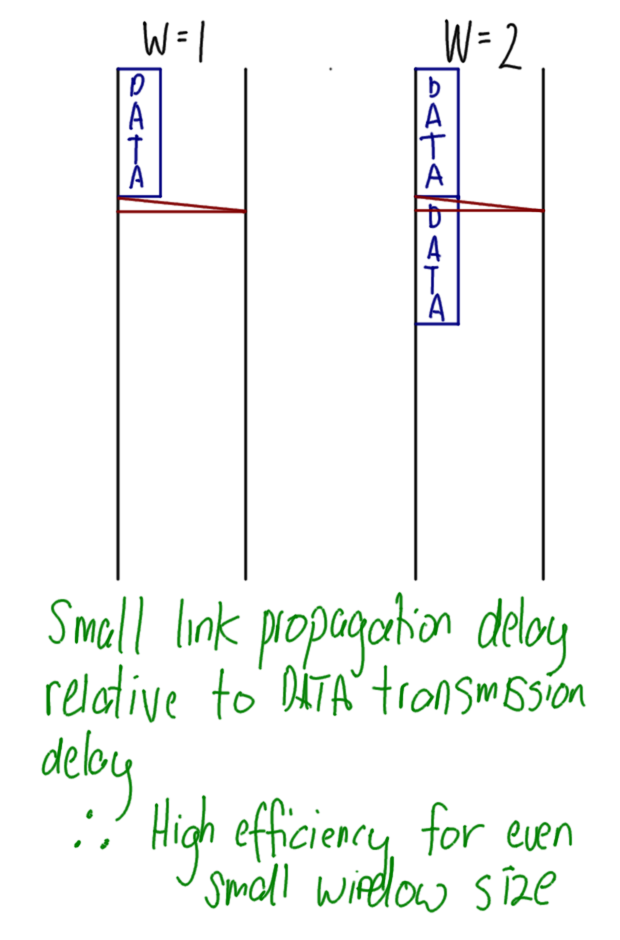
The efficiency will be high for W=1, and be maximum for W=2 (increasing W above 2 will not increase efficiency). These are BAD values of transmission and propagation times, because if you plot you may get something like:
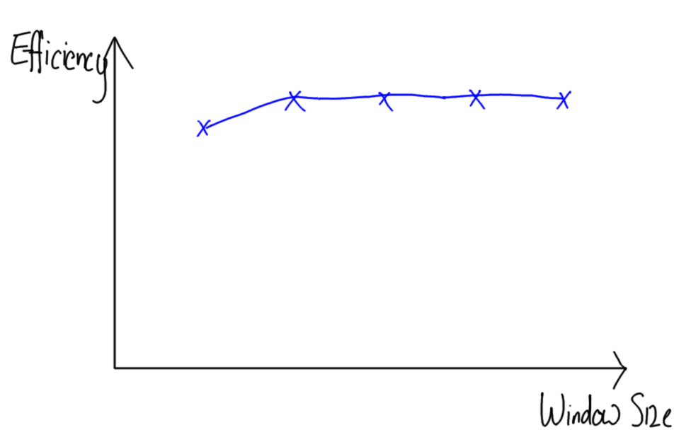
The efficiency does not change (much) as the window size changes.
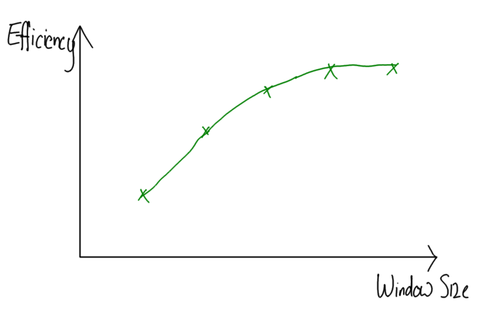
Now consider a different scenario where the transmission time is much smaller than the propagation time:
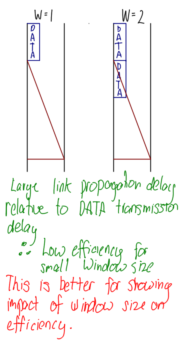
In this scenario you will get a wider range of efficiency values for different window sizes. Maybe the plot will look like:
This is a better scenario. In summary, make sure you choose the parameter values such that changing the window size causes a change in efficiency. The same applies for other parameters.
Finally, you should also plot the expected values alongside the measured values, and they should follow a similar pattern (they may not be identical though). Here is an example:
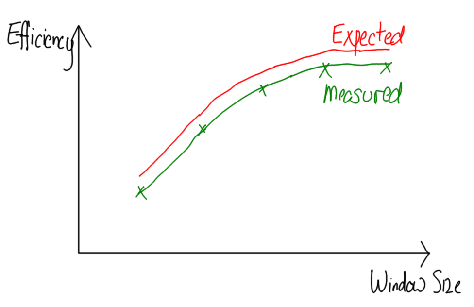
Maybe the best approach is to first plot the expected values, check that you see a significant change in efficiency, and then perform the experiments.
Finally, how many plots? You should produce a plot for each parameter you varied vs efficiency. For example, efficiency vs window size, efficiency vs data size, efficiency vs error rate, and so on. Again, there is no one correct answer as to the number of plots. If your report/experiments demonstrate that you have a good understanding of most (not necessarily all) tradeoffs involved with flow/error control then you can get full marks.
Each group submits three files:
Return to: Course Home | Course List | Steven Gordon's Home | SIIT